Dog Bark Detector - Machine Learning Model

Table of Contents

• Dog Bark Detector - Machine Learning Model
• Dog Bark Detector - Serverless Audio Processing
• Dog Bark Detector - Frontend

I've always been curious as to what my pets get up to when I'm out of the house. This curiosity finally got the best of me this week and I decided to build I wanted to build a dog bark detection system in order to keep track of how often our two dogs bark.

This guide covers the first of three guides around how the Dog Bark Detector was built; specifically focusing on the Machine Learning Model. You can see the components highlighted below that are core to this section of the guide.

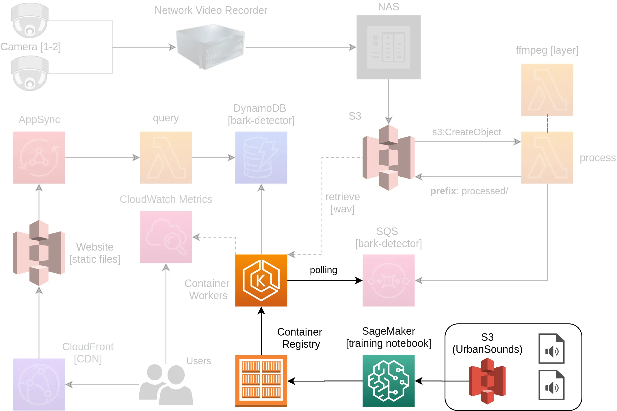
It covers the following concepts at a high level along with providing all the source code and resources you will need to create your own version.

• Researching existing solutions
• Data Collection from UrbanSound8K
• Model Training based on work by Mike Smales
• Dockerization of Model

Research

Before starting this project I wanted to make sure I wasn't reinventing the wheel. Having a reasonably good idea of what I wanted to achieve there was still some curiosity around how other people were going to go about solving this, so I hit the internet in search for some similar projects.

• tlynam/calm-barking-dog - An example of doing a series of audio filtering to detect the features common in dog barks. This project was promising however had a lot of issues getting it to run as it was over 6 years old now.
• nmkridler/sirbarksalot - Excellent example of an end to end solution doing analysis on an audio stream. The creator also demonstrated it at PyData Seattle 2017. Unfortunately the author didn't provide a model or dataset for me to use though.

After finding the two example above I knew that the method of converting the incoming audio files to spectrogram was likely the best approach, so with that knowledge in hand I narrowed by search down to a fantastic post by Mike Smales called Sound Classification using Deep Learning.

Not only was this post extensively detailed, but it also included links to the full dataset it was using. This dataset called UrbanSound8K contained 8732 sound excerpts that covered 10 different classes:

• Air Conditioner
• Car Horn
• Children Playing
• Dog bark
• Drilling
• Engine Idling
• Gun Shot
• Jackhammer
• Siren
• Street Music

Mikes code was also available at mikesmales/Udacity-ML-Capstone and included a ready made model fit for testing.

Data Collection

For this project I've re-purposed a lot of code provided originally by Mike Smales, the reinterpretation is available in t04glovern/dog-bark-detection.

NOTE: You are going to need to obtain a copy of the UrbanSound8K dataset from the 2014 release. Unfortunately an update to the dataset recently completely changed how it was formatted and accessed. Due to licensing reasons I cannot provide this dataset to you, but a quick google of it (look for a version that was approximately 6GB in size).

When working with the code in the t04glovern/dog-bark-detection repository you have two options:

• Pull down this repository locally and leverage Anaconda or Python
• Use Amazon SageMaker to run the notebook in the cloud.

Local Execution

The following steps can be run locally to pull down the repository and get the environment up and running

# Clone repository
git clone https://github.com/t04glovern/dog-bark-detection.git
cd dog-bark-detection

# Choice one of the following methods of setting up your environment
## Anaconda [preferred]
conda env create -f environment.yml
### If you are training on CPU, change `environment.yml`
### to use `tensorflow==1.14.0` instead
conda activate dog-bark

## Python
pip3 install --upgrade pip
pip3 install requirements.txt
pip3 install tensorflow-gpu==1.14.0 jupyter
### If you are training on CPU, install this instead
pip3 install tensorflow==1.14.0

With all the dependencies setup and ready to go, you can start Juypter notebooks using the following command

jupyter-notebook notebook.ipynb

You can now move onto the next step; skipping over the SageMaker setup given you are working locally.

SageMaker

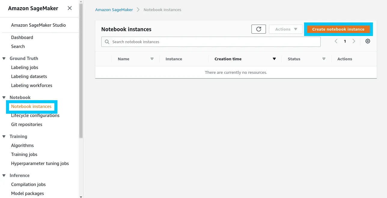
To run the repository on Amazon SageMaker navigate to the SageMaker console and click Create notebook instance under Notebook instances.

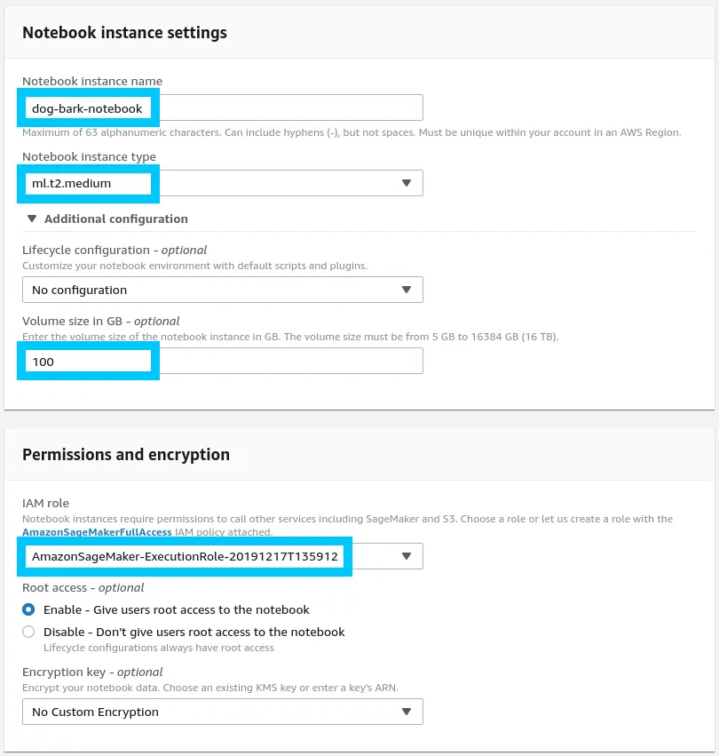
When creating a new SageMaker notebook there's a few specific settings we need to include.

• Notebook Disk Size changed to 100GB - This is because the dataset we are using is above the 5GB default for SageMaker projects.
• Create a new IAM role - Under Permissions and encryption create a new SageMaker access role using the guided prompt. If you want to provide access to any S3 buckets in your access then at this stage make sure to include those (the prompts will help you). Don't stress too much if you aren't too sure.
• Instance Type ml.t2.medium - We want accelerated compute, however it isn't technically necessary.

Scroll down and select to include a public repository as an optional setting for the notebook. This will allow you to include the Git repo for t04glovern/dog-bark-detection as part of the bootstrapping process.

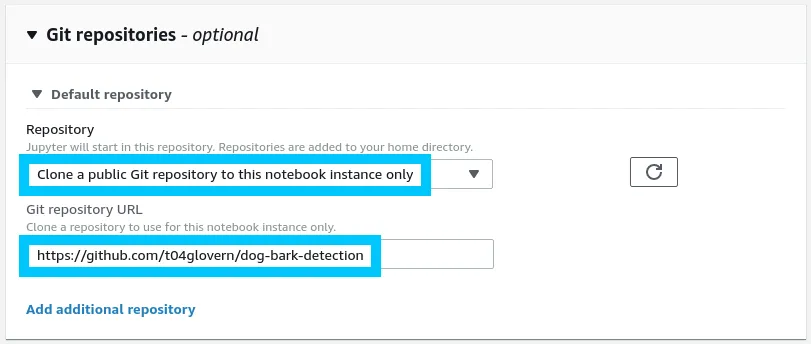
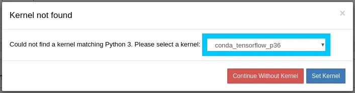
Click create repository and you in a couple minutes you should be able to access your new notebook from the SageMaker notebooks console. Once your SageMaker instance is accessible, open up the notebook.ipynb. If asked, set the Kernel for the notebook to be conda_tensorflow_p36.

NOTE: Since you are running on SageMaker you will also need to run and install the dependency cells before progressing.

Training Model

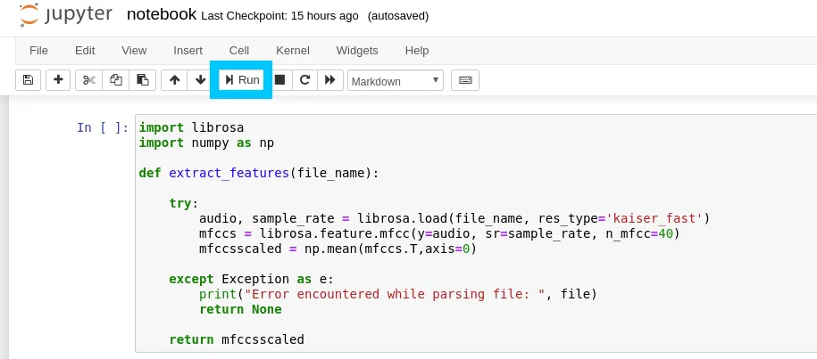
In the following section we will be executing each cell in our Jupyter Notebook one by one until we eventually have a fully trained model to perform inference against. The first few steps should already be completed prior to running the following sections:

• Dependencies - Should have been installed either via Anaconda, Python or within SageMaker
• Download & Unzip Dataset - Should be completed on your own as per instructions above downloading the UrbanSound8K dataset from the 2014 release.

Continue to click through each cell by clicking teh Run button. Each section should be pretty self explanatory based on the heading, however for extra context I again recommend checking out Mikes original code available at mikesmales/Udacity-ML-Capstone. He has fantastic descriptions that go in depth.

The longest process by far is loading in the Panda dataframe from the source dataset as this step requires the code to go through all ~8500 samples and load the features into a format that can be worked on.

# Load various imports
import pandas as pd
import os
import librosa

# Set the path to the full UrbanSound dataset
fulldatasetpath = './model/UrbanSound8K/audio/'
metadata = pd.read_csv('./model/UrbanSound8K/metadata/UrbanSound8K.csv')

features = []

# Iterate through each sound file and extract the features
for index, row in metadata.iterrows():
    file_name = os.path.join(
        os.path.abspath(fulldatasetpath),
        'fold' + str(row["fold"]) + '/',
        str(row["slice_file_name"])
    )
    class_label = row["class"]
    data = extract_features(file_name)
    features.append([data, class_label])

# Convert into a Panda dataframe
featuresdf = pd.DataFrame(features, columns=['feature','class'])

print('Finished feature extraction from ', len(featuresdf), ' files')

Eventually you will get down to the point where we can start training the model. In the code below feel free to tune the number of epochs (num_epochs) and batch size (num_batch_size); you might also feel like changing the output path of the model checkpoint to be somewhere other then model/wights.hdf5.

from keras.callbacks import ModelCheckpoint
from datetime import datetime

num_epochs = 100
num_batch_size = 32

checkpointer = ModelCheckpoint(filepath='model/weights.hdf5',
                               verbose=1, save_best_only=True)
start = datetime.now()

model.fit(x_train, y_train, batch_size=num_batch_size, epochs=num_epochs, validation_data=(x_test, y_test), callbacks=[checkpointer], verbose=1)

duration = datetime.now() - start
print("Training completed in time: ", duration)

When you run this cell you should start to see the training process kick off. Depending on the speed of your system it shouldn't take longer then a couple of minutes.

# Train on 6985 samples, validate on 1747 samples
# Epoch 1/100
# 6985/6985 [==============================] - 2s 253us/step - loss: 8.0705 - accuracy: 0.1828 - val_loss: 2.1634 - val_accuracy: 0.2158

# Epoch 00001: val_loss improved from inf to 2.16337, saving model to model/weights.hdf5
# Epoch 2/100
# 6985/6985 [==============================] - 1s 207us/step - loss: 2.2454 - accuracy: 0.2404 - val_loss: 2.0316 - val_accuracy: 0.2719

# Epoch 00002: val_loss improved from 2.16337 to 2.03159, saving model to model/weights.hdf5
# Epoch 3/100
# 6985/6985 [==============================] - 2s 221us/step - loss: 2.0285 - accuracy: 0.2953 - val_loss: 1.8351 - val_accuracy: 0.3795
# ...

Validation

The next step after model training is to perform some predictions using the weights we just generated. This can be done using the cells near the bottom of the notebook pretty easily

import librosa
import numpy as np

def extract_feature(file_name):
    try:
        audio_data, sample_rate = librosa.load(file_name, res_type='kaiser_fast')
        mfccs = librosa.feature.mfcc(y=audio_data, sr=sample_rate, n_mfcc=40)
        mfccsscaled = np.mean(mfccs.T,axis=0)
    except Exception as e:
        print("Error encountered while parsing file: ", file)
        return None, None

    return np.array([mfccsscaled])

def print_prediction(file_name):
    prediction_feature = extract_feature(file_name)

    predicted_vector = model.predict_classes(prediction_feature)
    predicted_class = le.inverse_transform(predicted_vector)
    print("The predicted class is:", predicted_class[0], '\n')

    predicted_proba_vector = model.predict_proba(prediction_feature)
    predicted_proba = predicted_proba_vector[0]
    for i in range(len(predicted_proba)):
        category = le.inverse_transform(np.array([i]))
        print(category[0], "\t\t : ", format(predicted_proba[i], '.32f'))

# Class: Dog Bark
filename = './model/bark.wav'
print_prediction(filename)

This should output a predicticted class of dog_bark, however your results might vary.

The predicted class is: dog_bark

air_conditioner     :  0.00007508506678277626633644104004
car_horn            :  0.00194400409236550331115722656250
children_playing    :  0.15097603201866149902343750000000
dog_bark            :  0.83962621688842773437500000000000
drilling            :  0.02223576419055461883544921875000
engine_idling       :  0.00090576411457732319831848144531
gun_shot            :  0.37796273827552795410156250000000
jackhammer          :  0.00000017495810311629611533135176
siren               :  0.00116558570880442857742309570312
street_music        :  0.00510869221761822700500488281250

Before moving on, make a copy of your model/wights.hdf5 for future use in the following inference step.

IMPORTANT NOTE: Be sure to switch off (and delete) your SageMaker notebook once you have finished using it, as the one we were using costs $2 an hour.

Inference

Now that I had a working model and some basic code that could be used to retrieve results from a WAV file input, I now needed to package all this up as a service. With this in mind I decided to take a page out of a book written in the past for selfie2anime where we had images sent to Amazon S3 (File Store) and processed using Amazon Simple Queue Service (SQS).

The code for this part can be found in the main.py file in the root of the t04glovern/dog-bark-detector project. The implementation details will make a little bit more sense when exploring the next post Dog Bark Detector - Serverless Audio Processing, however for now all you need to know is:

• WAV files are saved to Amazon S3
• SQS Queue receives item pointing to a new set of WAV files to process
• Inference code pulls down WAV files and runs inference on each one
• If a dog bark is detected an entry is added to Amazon DynamoDB

All of this logic needed to be bundled up in a package that could be scaled out to multiple workers, so I decided to dockerize the project. Check out the Dockerfile below to get an understanding of how this was achieved

FROM tensorflow/tensorflow:1.14.0-gpu-py3

RUN apt-get update && apt-get install ffmpeg libsndfile1 -y

COPY . /app
WORKDIR /app

RUN pip3 install -r requirements.txt

ENTRYPOINT [ "python3" ]
CMD [ "main.py" ]

docker-compose

If you would like to try running this service locally, I've created a docker-compose.yml file that will assist in injecting the required environment variables and building the container for you. You will likely need to change the QUEUE_NAME and TABLE_NAME based on your setup (learn more about this in the next guide).

# Bring service up
docker-compose up

# Take service down
docker-compose down -v

Conclusion

This concludes the first part of this guide where we've achieved our goal of creating a Dog Bark detector model using Keras, UrbanSound8K and Amazon SageMaker. If you enjoyed this guide and would like to continue along building out this solution, check out the next guides in the series:

• Dog Bark Detector - Serverless Audio Processing
• Dog Bark Detector - Frontend

If you have any questions or want to show off your models results; please hit me up on Twitter @nathangloverAUS